Satellite Image Correction Models

Satellite data are made available to the science team in calibrated at-sensor radiance units (W str-1 m-2 s-1) as spatially contiguous orthorectified mosaics. These data require extensive processing using GDCS algorithms to generate at-surface, sub-surface, and benthic reflectance data from the Planet radiance imagery. Reaching these three levels of processed data requires modeling of the radiometry of each Planet satellite (Dove, SkySat) used in generating coral reef coverage worldwide. Additionally, the following corrections need to be applied to Planet data to support the UQ mapping component (geomorphic zonation and benthic composition) as well as the GDCS alert-monitoring component:

Atmospheric correction

The corrections for both the atmospheric effect and water column attenuation derive the benthic reflectance (or bottom reflectance). The derived benthic reflectance is applied to the coral reef classification and bleaching detection with improved accuracy. The method was developed based on the four bands (B, G, R, and near infrared [NIR]) Planet Dove satellite images for deriving the benthic with the assistance of depth data.

Waterbody retrieval

Ocean region is delineated from the corrected satellite images through the normalized difference water index as:

Then the following processing is processed on the water-only region.

Sun glint removal

The removal of sun glint (water surface effect) in the study regions were performed by equation 1 as:

Where Rrs, 0+ is the remote sensing reflectance just above the water surface in blue, green and red bands, Rrs is the water leaving reflectance (R, G and B), and Rrs(NIR) is the reflectance in the NIR band. After the sun glint correction, the below surface reflectance is derived as:

Depth calculation

A band-ratio algorithm is applied for deriving the depth based on B, G, and R bands of the Dove images:

The tunable constant (m0 and m1) is calibrated for the study sites according to the water column attenuation conditions. this research was supported by The Nature Conservancy

For validation of the water depth product, reference data from field measured water depths is compared with coincident locations on the map product and to calculate regression values. Field measured depth is sourced from previously collected data from existing programs.

Bottom Reflectance estimation

In optically shallow waters, the water-leaving reflectance is made up of contributions from both waterbody and bottom sediments. So the below-surface remote sensing reflectance rrs is modeled as:

where r^c_rs represents the water column contribution. r^b_rs represents the bottom sediments contribution at below-water surface. H is the estimated depth, and B is the bottom reflectance to be derived. D(a_t+b_b) represents the light attenuation caused by water column absorption and backscattering for water column light components (D_c) or light components from bottom (D_b).

Finally, D_c and D_b are empirical factors associated with under-water photon path elongation due to scattering and are calculated as below:

r^rs_dp represents below-surface remote sensing reflectance when the water is infinitely deep and is modeled as:

Then the water inherent optical properties (IOPs) are modeled as different components of water as:

The water IOPs contain the contribution of pure water ( a_w(λ ), b_bw(λ) ), CDOM ( a_cdom(λ ) ) and particles ( a_p (λ) , b_bp(λ) ). Then the bottom reflectance can be derived.

Diagrammatic workflow from Dove reflectance to derive the depth and bottom reflectance. The different components are illustrated below as the methodology sections above. The normalized difference water index (NDWI) is applied to mark water and land regions.

For the water regions, the sun glint (or water surface effect) is removed by subtracting the NIR band. The water leaving signals ( R_rs ) are then derived. Next, the subsurface remote sensing reflectance is calculated to remove the sea-air interface effect. Finally, the water column attenuation correction is processed

References

Gao, Bo-Cai. 1996. “NDWI—A Normalized Difference Water Index for Remote Sensing of Vegetation Liquid Water from Space.” Remote Sensing of Environment 58 (3): 257–66.

Lee, ZhongPing, Kendall L. Carder, and Robert A. Arnone. 2002. “Deriving Inherent Optical Properties from Water Color: A Multiband Quasi-Analytical Algorithm for Optically Deep Waters.” Applied Optics 41 (27): 5755–72.

Lee, Zhongping, Kendall L. Carder, Curtis D. Mobley, Robert G. Steward, and Jennifer S. Patch. 1999. “Hyperspectral Remote Sensing for Shallow Waters. 2. Deriving Bottom Depths and Water Properties by Optimization.” Applied Optics38 (18): 3831–43.

Lee, Zhongping, Alan Weidemann, and Robert Arnone. 2013. “Combined Effect of Reduced Band Number and Increased Bandwidth on Shallow Water Remote Sensing: The Case of Worldview 2.” IEEE Transactions on Geoscience and Remote Sensing51 (5): 2577–86.

Li, Jiwei, Qian Yu, Yong Q. Tian, and Brian L. Becker. 2017. “Remote Sensing Estimation of Colored Dissolved Organic Matter (CDOM) in Optically Shallow Waters.” ISPRS Journal of Photogrammetry and Remote Sensing 128: 98–110.

Wabnitz, Colette C., Serge Andréfouët, Damaris Torres-Pulliza, Frank E. Müller-Karger, and Philip A. Kramer. 2008. “Regional-Scale Seagrass Habitat Mapping in the Wider Caribbean Region Using Landsat Sensors: Applications to Conservation and Ecology.” Remote Sensing of Environment 112 (8): 3455–67.

Bathymetry

This bathymetry product was developed by the Allen Coral Atlas team. Shallow water bathymetry is mapped in centimeters. There are several steps in the data processing that are outlined below.

Data Properties

The bathymetry maps are created at a resolution of 10 m using the Google Earth Engine (GEE) Sentinel-2 surface reflectance dataset. Sentinel-2 satellite images with minimal cloud coverage and turbid water over 12 months are selected. The input dataset is aggregated into a single clean mosaic output using the median depth value over 12 months. In the area without sufficient Sentinel-2 coverage, Landsat-8 and Planet Dove satellite images are used to derive depth and produce a composite image from the 3 datasets.

Methods

We developed a new automatic bathymetry mapping method based on a previous single-scene adaptive bathymetry algorithm (Li et al., 2019). Our algorithm was tailored to the clean water mosaic built by GEE. We first calculated remote sensing reflectance  from the mosaic surface reflectance (ρ(λ)) as:

Next, we derived below-surface remote sensing reflectance () from the ( to remove the air-water surface effect:

We estimated shallow water bathymetry by quantifying different attenuation levels between the blue and green bands as:

The bathymetry estimation parameters ( and ) were calculated using a Chlorophyll-a (Chl-a) concentration value as a representative for clean offshore waters:

As noted previously, we only selected satellite images with low water turbidity to build the mosaic. Also, given that the water mosaic values represent the median value over time (i.e., 12 months), we used a fixed Chl-a value to calculate  and  in our clean shallow water mosaic. This Chl-a value is a mean value calculated from GEE outputted clean water mosiac in 26 sites globally.

Data Download

The bathymetry products are downloadable. Bathymetry maps show the satellite derived bathymetry values where the bottom is visible in satellite images. The bathymetry image is stored as a GeoTIFF file. Each pixel in the bathymetry image is represented by a 16-bit integer.

References

Li, J., D.E. Knapp, S.R. Schill, C. Roelfsema, S. Phinn, M. Silman, J. Mascaro, and G.P. Asner*. Adaptive bathymetry estimation for shallow coastal waters using Planet Dove satellites. Remote Sensing of Environment, 232 (2019).

Li, J., D.E. Knapp, M. Lyons, C. Roelfsema, S. Phinn, S.R. Schill, G.P. Asner*. Automated global coastal water bathymetry mapping using Google Earth Engine. (in review)

Reef Extent

As part of the Allen Coral Atlas’s revisions to its habitat maps in 2022, a new reef extent product was generated for each mapping region. This is intended to provide a more generalized and inclusive layer that depicts the extent of the coral reef environment which is additional to the Atlas’ geomorphic zonation maps.

Definition

Reef extent definition: In context of this product, reef extent is defined as the location of shallow coral reef features that can generally be seen from satellites. It typically excludes areas of very deep and very turbid water.

Methods

The underlying reef extent product is a raster at 5m pixel resolution, matching the geomorphic and benthic map products. The raster combines three sources:

1. The extent of the Allen Coral Atlas’s 12 geomorphic zones

2. The extent of our own machine learning-based coral reef habitat layer, originally developed for the Global Coral Reef Monitoring Network’s 2020 Report on the Status of Coral Reefs of the World

3. A third extent layer that:

   1. Filled in holes greater than 400 pixels (0.64Ha)

   2. Applied a morphological filter (circle kernel of 5 pixels; 25m) to smooth the reef boundaries and regain missing slope/beach features

For the purposes of the data product made visible on the Allen Coral Atlas, these three sources are combined into one single-colored layer.

Features

The reef extent layer more inclusively depicts the shallow coral reef environment than our more detailed benthic or geomorphic habitat maps. It includes reef features that were unmappable to geomorphic/benthic level, including deeper reef structures, reef habitat in more turbid water, deep or very steep reef slope areas, and very shallow intertidal areas at the land-sea interface. Known limitations are that some areas of supra-tidal beach and vegetation are included, which may not strictly be coral reef environments. Overall, the reef extent product is still conservative, and we expect that the area of reef erroneously included at the land-sea interface is greatly outweighed by the areas of reef still missed at both the shallow and deep margins of the product.

Visualization

The reef extent data product can be seen as a single layer on the Atlas and compared and analyzed alongside other datasets such as reef habitat maps and reef threat monitoring datasets. 

Habitat Mapping

Classification Scheme

To map geomorphic and benthic zones of global coral reefs we use Planet Dove image data, water depth derived from Sentinel 2, Landsat or Planet Dove satellite imagery, modelled waves and surrogates for texture and slope through machine learning random forest classification followed by an object based cleaning approach using eco-geomorphological rules.

Coral reefs can be conceptually organised into four levels of physical and biological structure (Figure 1), and the global coral reef mapping in the Coral Atlas focusses on geomorphic zonation and benthic composition (Figure 2). Specifically, these layers are:

1. Reef geomorphic zonation (mapped to ~ 15 m deep) – classification within individual reefs into zones
2. Reef benthic composition (mapped to ~10 m deep) – classification within reef zones into habitats
   
   

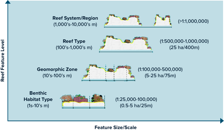
Figure 1: Minimum mapping units, spatial scale and levels of mapping detail to be used for coral reefs

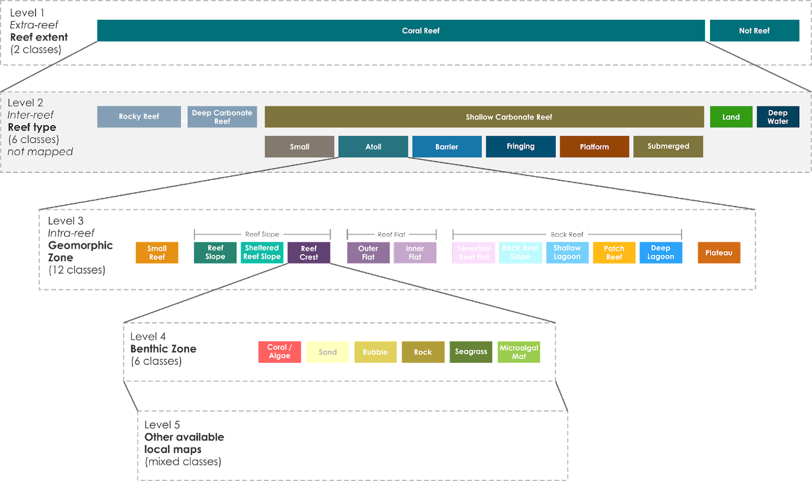
Figure 2: Allen Coral Atlas mapped classes. Coloured boxes represent map classes used in the hierarchical classification scheme applied in the project.

The Allen Coral Atlas classification scheme outlined in Figure 1 and Figure 2 forms the backbone of the Allen Coral Atlas (Kennedy et al. 2021). Classes were also designed with users in mind to reflect ecological, geological and socially meaningful features of reefs, and constrained by mapping capability with input data available and the approach followed, for more detail see(Kennedy et al. 2021). Development of mapping classes required a sensitive trade-off between the requirements of users in terms of the level of detail needed, the input resources available and the quality of the globally repeatable mapping methods. Our classes paid respect to  recent regional to global scale coral reef mapping projects (e.g. NOAA maps), as well as other past global projects and current NOAA UNEP global coral data sets were reviewed. Detailed descriptions of geomorphic and benthic classes can be found for the Allen Coral Atlas.

Mapping Regions

The scale of the project, computational power needed and regional inconsistencies in coral reef structure and size meant that a region-by-region approach to mapping the worlds reefs was adopted (Figure 3). Mapping regions include reef areas that fall between the 30 degrees latitude and in clear shallow waters (less then approximately 20 m deep) that would be amenable for satellite based information extraction. Regions were derived from a combination of existing global bio regionalisation’s that account for coral biogeography (Veron et al. 2016.) and oceanography (Spalding et al. 2007) modified based on visual assessment of reef areas observed on the dove satellite image mosaic, the reef types, water depth and water quality to result in 30 regions.  

Figure 3: Allen Coral Atlas mapping methodology relies on a region-by-region approach to mapping the world's reefs. The target mapping regions (pictured) reflect established patterns of coral reef biogeography, with similar reef type, environmental conditions and do not consider geo-political boundaries.

The mapping region outline was then combined with a global reef satellite scene mask to create mapping region specific mask. A global potential reef satellite scene mask was initially created to reduce the area for which Dove imagery has to be acquired and manage the computational efforts. The reef scene mask included areas: within the 30 degrees latitude; shallower then 20 m by creating a buffer around the approximately 20 m depth sourced from an existing course level global depth layer; not included land using a global land outline; and have a known presence of reefs using the UNEP-WCMC Coral Reef Layer 2018(UNEP-WCMC et al. 2018). The global reef scene mask was finalized by visual based contextual editing using a global Landsat mosaic. 

Geomorphic and Benthic Mapping Principles

The current geomorphic and benthic mapping approach combines machine learning with Object Based Analysis (OBA)(Lyons et al. 2020) (Figure 5).  It includes four modules: 1) Data Preparation, 2) Machine Learning Classification, 3) OBA clean-up and 4) Accuracy Assessment.

Figure 3: Flow chart detailing the four key modules of the coral reef mapping framework, including the data input types, processing steps and output products (Lyons et al. 2020). 

Module 1. Data Preparation

In Module 1 the input data sets and reference samples are prepared for Module 2, the machine learning component.

The input data sets include: Planet satellite image mosaic, physical attributes including water depth from Sentinel 2, Landsat 8, Planet Dove data (Li et al. 2019), exposure to waves (Harris et al in prep), turbidity (Li et al in prep), and reference samples for training and validation purpose.

The satellite image and physical attribute data are segmented into ‘objects’ following an OBA paradigm (Lyons et al. 2020), and the segmented information is added to the ‘data stack’ so that both local and neighbourhood information can inform the mapping process. The OBA paradigm is based on the image and other spatial data to be first segmented into groups of pixels with similar characteristics (e.g. colour or texture, or a physical property such as water depth). This is akin to how we use our eyes to segment images into objects for interpretation. Each image ‘object’ is given a set of metrics based on its constituent pixels – in this case we use the mean values for each of the metrics in the pixel-based data stack.

Reference Samples: Training and validation data (point-based) are used to train the machine learning classifier and validate the resulting maps. These points are derived from as a large pool of reference samples and then randomly split into training and validation. Reference samples (objects) are created by assigning mapping classes to a subset of objects for small representative groups of reefs within a mapping region (Roelfsema et al. 2021). Assigning labels to reference samples, is currently based on manual labelling of segments by a trained expert. The trained experts would visually review: a combination of classification description that include class typology (Kennedy et al. 2021); satellite image colour and texture; depth and waves; existing coral reef habitat maps, existing or new field data and expert knowledge. All reference samples are available Where the existing and newly collected or created field data or maps are provided through the verification component of the Allen Coral Atlas, described in detail in methods section.

Module 2. Machine Learning Classifier

Using a training data set, a machine learning Random Forest classifier is used to make a preliminary classification of geomorphic and benthic classes. The Random Forest classifier is a well-established machine learning algorithm used to create maps from the data. It is an ‘ensemble learning’ method, which means it assesses the input data based on a number of constructed ‘decision trees’, that each have a component of random variation in the parameterisation. The final decision takes into account all of the different possibilities in the different decision trees. and they are particularly useful because they balance predictive performance with overfitting, and are also robust to redundant predictor variables (James et al. 2013). The classifier is trained used the curated training data set, with the input variables (e.g. mean band values, depth, waves) included both the pixel and segmented objects from the image and physical environment data.

Module 3. Object Based Clean Up

Based on an established framework for OBA on the Great Barrier Reef (Roelfsema et al. 2018, Roelfsema et al. 2020), the preliminary classification is then refined using the contextual principles of OBA. The output classification from the machine leaning classifier is then processed using a number of automated OBA membership rules. Membership rules form the typology of a mapping class defined by different attributes or spatial relationships. These attributes are typically based on contextual information based on where a class is, its attributes (e.g. depth, waves) and what its neighbouring classes are. For example, a generic rules could be if Class A (e.g. Reef Crest) is small and surrounded by class B (e.g. Outer Reef Flat) then Class A should be reclassified to B. This module includes a component where additional relationship rules and/or mask are created to improve the maps.

Module 4. Accuracy Assessment and Confidence Levels

Accuracy Measures and Error Matrix

Validation points were derived from the reference samples, and then compared with the mapped data through an error matrix. From the error matrix standard accuracy measures were derived that include overall map accuracy and the individual map category user and producer accuracy (Congalton et al. 2008).

Wave Climate Model

Wave exposure is the dominant force influencing the ecological makeup and physical structure of coral reefs. Changes in the benthic ecological community as well as some crucial metabolic and biological functions of coral reefs have been linked to variations in wave energy. Long-term geomorphic development of coral reefs is also driven by the relative exposure of coral reefs to wave processes. A thorough understanding of wave exposure is now an important component of benthic ecological surveying in coral reefs. Wave exposure on coral reefs has typically been determined  using a suite or computationally onerous models which limits wave modelling to a local or regional basis which. To calculate the wave exposure for every reef in the world a wave model that is flexible, computationally fast and links with global wave models. This model uses principles of wave refraction and diffraction to determine the dissipation of wave energy from deepwater sources to shallow reef environments and through often complex coral reef regions. This provides the local wave height for every reef prior to wave breakpoint and hence the wave exposure index for each coral reef.
Datasets: National Oceanic and Atmospheric Associate (NOAA) Wave Watch III global wave model hindcast reanalysis (1979-present). Global bathymetry.

Software Used 

Reference samples are created with the help commercial software Trimble eCognition 9.3. in the Allen Coral Atlas workflow. The machine learning mapping and the  For the mapping regions, the machine learning and OBA refinement stages are implemented in Google Earth Engine, and open source and free cloud-based processing environment that provides capability to access and process the Planet Dove imagery, along with a range of other satellite image archives (e.g. Sentinel 2, Landsat). The image segmentation and OBA refinement workflow was not previously available in Google Earth Engine, so that software capability is a major output of the Allen Coral Atlas project (Lyons et al. 2020).

For more information on mapping and monitoring through remote sensing from the University of Queensland, check out this Remote Sensing Toolkit

Reference

Congalton, R. G. and K. Green (2008). Assessing the accuracy of remotely sensed data: Principles and practices. Mapping Science. Boca Rotan FL, CRC Press.

James, G., D. Witten, T. Hastie and R. Tibshirani (2013). An introduction to statistical learning. New York, Springer.

Kennedy, E., C. M. Roelfsema, M. B. Lyons, E. Kovacs, R. Borrego-Acevedo, M. Roe, S. R. Phinn, K. Larsen, N. Murray, D. Yuwono, J. Wolff and P. Tudman (2021). "Reef Cover, a coral reef classification for global habitat mapping from remote sensing." Scientific Data.

Li, J., D. E. Knapp, S. R. Schill, C. Roelfsema, S. Phinn, M. Silman, J. Mascaro and G. P. Asner (2019). "Adaptive bathymetry estimation for shallow coastal waters using Planet Dove satellites." Remote Sensing of Environment 232: 111302.

Lyons, M., C. Roelfsema, V. E. Kennedy, E. Kovacs, R. Borrego-Acevedo, K. Markey, M. Roe, D. Yuwono, D. Harris, S. Phinn, G. P. Asner, J. Li, D. Knapp, N. Fabina, K. Larsen, D. Traganos and N. Murray (2020). "Mapping the world's coral reefs using a global multiscale earth observation framework." Remote Sensing in Ecology and Conservation n/a(n/a).

Roelfsema, C., E. Kovacs, J. C. Ortiz, N. H. Wolff, D. Callaghan, M. Wettle, M. Ronan, S. M. Hamylton, P. J. Mumby and S. Phinn (2018). "Coral reef habitat mapping: A combination of object-based image analysis and ecological modelling." Remote Sensing of Environment 208: 27-41.

Roelfsema, C. M., E. M. Kovacs, J. C. Ortiz, D. P. Callaghan, K. Hock, M. Mongin, K. Johansen, P. J. Mumby, M. Wettle, M. Ronan, P. Lundgren, E. V. Kennedy and S. R. Phinn (2020). "Habitat maps to enhance monitoring and management of the Great Barrier Reef." Coral Reefs.

Roelfsema, C. M., M. Lyons, N. Murray, E. M. Kovacs, E. Kennedy, K. Markey, R. Borrego-Acevedo, A. Ordoñez Alvarez, C. Say, P. Tudman, M. Roe, J. Wolff, D. Traganos, G. P. Asner, B. Bambic, B. Free, H. E. Fox, Z. Lieb and S. R. Phinn (2021). "Workflow for the Generation of Expert-Derived Training and Validation Data: A View to Global Scale Habitat Mapping." Frontiers in Marine Science 8: 228.

Spalding, M. D., H. E. Fox, G. R. Allen, N. Davidson, Z. A. Ferdaña, M. Finlayson, B. S. Halpern, M. A. Jorge, A. Lombana, S. A. Lourie, K. D. Martin, E. McManus, J. Molnar, C. A. Recchia and J. Robertson (2007). "Marine Ecoregions of the World: A Bioregionalization of Coastal and Shelf Areas." BioScience 57(7): 573-583.

UNEP-WCMC, WorldFish Centre, WRI and TNC (2018). Global distribution of warm-water coral reefs, compiled from multiple sources including the Millennium Coral Reef Mapping Project. Version 4.0. . U. E. W. C. M. Centre, Cambridge (UK): .

Veron, J. E. N., M. G. Stafford-Smith, E. Turak and DeVantier. L. (2016.). "Corals of the World." from http://coralsoftheworld.org.

Coral Reef Watch

Coral Reef Watch (NOAA NESDIS)

The Coral Reef Watch near real-time 5km global products on the Allen Coral Atlas site are the most recent day's published sea surface temperature (SST), SST Anomaly, Coral Bleaching HotSpot, Degree Heating Week (DHW), a 7-day maximum Bleaching Alert Area, and 7-day SST Trend data from NOAA's Coral Reef Watch program. Please see their website for more information about the program. For more technical details about the 5-km products, see Liu et al. 2017 and 2014, and Heron et al. 2016 and 2015. If these products are used in any way, please follow the citation guidance.

Coral Reef Bleaching Monitoring

The monitoring of apparent bleaching coral relies upon the initial indication of bleaching threat by marine heatwaves.  The National Oceanic and Atmospheric Administration Coral Reef Watch (NOAA-CRW) program records daily sea surface temperature (SST) anomalies. These data are used to indicate a level of warning for coral reef bleaching for 214 coral regions around the globe.  When a region enters a level of “Bleaching Alert Level 1” or higher in the NOAA system, the Allen Coral Atlas initiates its own processing of Sentinel-2 satellite data for that region on a bi-weekly basis. Conversely, when a region goes back to “No Stress” or the Degree Heating Weeks decreases to 0.5 or below in the NOAA system, the Allen Coral Atlas system stops monitoring that region.

Figure 1. Example of Fiji Sea Surface Temperature data during 2022-2023

Methods

To monitor a region that is under a NOAA bleaching alert, we first establish the median baseline bottom reflectance during a period when the region is not under thermal stress. This is during a period of cool water temperatures. The baseline is built with the consecutive 42-days data available prior to the region reaching the Bleaching Warning thermal stress. If over this time the region experiences short Bleaching Warning thermal stress intervals, the baseline is pushed backwards and built with the 42-days prior to that. This process can be repeated up to 180 days before the monitoring starts. The satellite data are masked with Google Earth Engine (GEE) using the QA60 and Scene Classification Map (SCL) bands of Sentinel-2 data to remove pixels with clouds, shadows, and other disturbances. The image collection is then processed by using the Median Reducer in GEE in order to get a clean surface reflectance image. In addition to the median surface reflectance, we also calculate the standard deviation of the reflectance to establish the level of natural variation that a pixel may experience, independently of the  thermal event. The median surface reflectance image generated from Sentinel-2 data is then converted to bottom (seafloor) reflectance as described in Li et al. (2020) (Figure 2).  This method uses water depth as an input along with the inherent optical properties (IOPs) of the water column. The depth data are also derived from the Sentinel-2 imagery as described by Li et al (2021).  The chlorophyll-a concentration (Chl-a) is required to estimate the total absorption and scattering coefficients of the water column, since it is used in the calculation of the phytoplankton absorption coefficient (Lee, Weidemann, and Arnone, 2013) and the particle backscattering coefficient (Morel and Maritorena, 2001). For this, the Chl-a was derived from the above surface remote sensing reflectance (Hu, Lee, and Franz 2012), and the regional average Chl-a between June 2020 and December 2021 was calculated and used in the calculations.

Figure 2. Flowchart of processing and compilation of bi-weekly data for identifying areas of possible brightening.

For each thermal event, we depend on the comparison of two images. The first one is the baseline image built as described earlier.  The second image is created by collecting the median surface reflectance image for a 2-week period after the monitoring starts (Figure 3).  We apply the same masking and bottom reflectance algorithms to the Sentinel-2 data for each 2-week period of monitoring. Each bi-weekly mean bottom reflectance is then compared to the bottom reflectance baseline image to identify when a pixel is above the baseline median plus one standard deviation. By counting the number of times (i.e., number of 2-week intervals) a pixel is above this threshold (Figure 2), the bleaching persistence value (PV) is built. Through the PV we infer whether the brightening of a pixel is linked to a bleaching event or not. The resulting pixel count is masked so that only the pixels in the “coral/algae” benthic class from the Allen Coral Atlas are included.

Figure 3.   

The pixel counts are clustered into classes of low, moderate, and severe bleaching. The pixel counts indicate the number of 2-week intervals that a pixel is brighter than one standard deviation above the median bottom reflectance from the baseline period. The threshold is set to be fairly conservative and can be adjusted as we receive feedback from observers in the field.  Because of the potential for some pixels to be brighter as a result of anomalies that are not caught in the masking steps, we set the interpretation of the values such that a value of two (i.e. 2 two-week periods) will be the lowest value of possible bleaching (Low level of bleaching).  As the more two-week periods pass, if the same area continually registers above the threshold, the PV will increase.  A value of four is indicative of a Medium level of bleaching and 6 or higher is the most Severe level.  
The monitoring of a region stops either when “No stress” is encountered or when the Degree Heating Weeks decrease to 0.5 or below. After every bleaching period finishes, a recovering period is established, raising the eight weeks following the end of the event. Throughout this time, and 42 days +, the region is not monitored.
This is our bleaching method as of April 2023. Prior to this date, the monitoring system was activated by the heat stress level “Bleaching Warning” of the NOAA system, one category lower than the one used in the new version. In addition, the end of the monitoring was determined by only reaching “No Stress” level. A major change in the new monitoring system is the baseline definition, as in the previous version it was built with the satellite data from the 3-month period when the lowest sea surface temperature was registered in the last 410 days. This methodology used to allow using the same baseline to more than one event in the same year. At last, as it was mentioned before, in the new version a set of regional Chl-a values are used, while in the previous version a mean value of 0.5 mg/m3 was used for all the regions, which misrepresented the spatial variability of that water component. The entirety of our original methods can be found here. 

References

1. NOAA Coral Reef Watch. 2021, updated daily. NOAA Coral Reef Watch Version 3.1 Daily 5km Satellite Regional Virtual Station Time Series Data.  College Park, Maryland, USA: NOAA Coral Reef Watch. Data set accessed 2021-04-13 at https://coralreefwatch.noaa.gov/product/vs/data.php.

2. Li, J.; Fabina, N.S.; Knapp, D.E.; Asner, G.P. The Sensitivity of Multi-Spectral Satellite Sensors to Benthic Habitat Change. Remote Sens. 2020, 12, 532.

3. Li, J.; Knapp, D.E.; Lyons, M.; Roelfsema, C.; Phinn, S. Schill, S.; Asner, G.P.  Automated Global Shallow Water Bathymetry Mapping Using Google Earth Engine. Remote Sens. 2021, 13, 1469.

4. Lee, Z.; Weidemann, A.; Arnone, R. Combined Effect of Reduced Band Number and Increased Bandwidth on Shallow Water Remote Sensing: The Case of WorldView 2, IEEE Transactions on Geoscience and Remote Sensing, May 2013, vol. 51, no. 5, pp. 2577-2586, doi: 10.1109/TGRS.2012.2218818.

5. Morel, A., and Maritorena, S. Bio-optical properties of oceanic waters: A reappraisal, J. Geophys. Res. 2001 106( C4), 7163– 7180, doi:10.1029/2000JC000319.

6. Hu, C.; Lee,  Z.; Franz, B. Chlorophyll a algorithms for oligotrophic oceans: A novel approach based on three-band reflectance difference, J. Geophys. Res 2012, 117, C01011, doi:10.1029/2011JC007395.

Turbidity

This annual water turbidity product was developed by the ASU scientific team of the Allen Coral Atlas. Water turbidity levels are commonly represented by Formazin Nephelometric Units (FNU). The downloadable turbidity maps are multiplied by 10 to be stored in a 16-bit integer format. Therefore, downloadable turbidity maps are in (FNU*10) units. For instance, a value “55” in the turbidity maps is “5.5 FNU”. The maximum detectable turbidity value is 100 FNU. There are several steps in data processing that are outlined below.

Data Properties

The annual basemaps are created at a resolution of 10 m using the Google Earth Engine Sentinel-2 surface reflectance dataset. Sentinel-2 satellite images with minimal cloud coverage and sun glint over three months are selected. The input dataset is aggregated into a single mosaic output to calculate the median turbidity value from the calendar year.

Methods

We applied a Shallow Water Turbidity (SWaT) estimation algorithm in clean reef water regions to account for the effects of bottom reflectance and to derive accurate turbidity measurements (Li et al, 2022). In optically-deep waters (e.g., high turbidity river plume regions), we applied an optically-deep turbidity algorithm (Dogliotti et al, 2015). In SWaT, water turbidity (T) was calibrated using field-measured turbidity worldwide by using two wavelength-dependent calibration coefficients (i.e.,  ) as:

 is water-leaving reflectance. Both  and  are wavelength-dependent calibration coefficients which are calculated in different wavelengths as a global applicable model.

In shallow coastal waters, the water-leaving reflectance ( ) is calculated from the contribution of both water column ( ) and bottom reflectance ():

where H is water depth,   is water-column attenuation, and   is bottom reflectance. So, water-column remote sensing reflectance ( ) was calculated in the SWaT as:

Turbidity in shallow coastal waters () was calculated as:

We introduced the bottom reflectance contribution () to abbreviate bottom effects in the turbidity calculation (Li et al., 2022). We applied the value of (= 268.52) and ( = 0.1725) based on the central wavelength of Sentinel-2’s red band, which is calibrated in the previous studies as a global applicable model.

The following image shows the turbidity product’s calculation steps:

Data Download

The turbidity products are downloadable. Downloaded annual turbidity maps show the median turbidity value over a twelve-month period, which help to identify and detect the annual turbid waters hotspots over coral reefs and associated water environments. Downloaded turbidity products will appear different from what is represented graphically on the Atlas because of the visual transformations discussed below in “Visualization”.

Visualization

We produced the turbidity maps visible in the Atlas by reducing the computed turbidity values to six possible bins representing minimal turbidity (values <= 45 (4.5 FNU)), low turbidity (<= 52 (5.2 FNU)), moderate turbidity (<= 58 (5.8 FNU)), high turbidity (<= 66 (6.6 FNU)), severe turbidity (<= 79 (7.9 FNU)), and extreme turbidity (> 79 (7.9 FNU)).  These bins equate to the 6-quantiles of the distribution of over 780 trillion turbidity pixel values computed across tropical coral reef habitat areas globally from 2019 through 2023.  We smoothed the binned turbidity representation with a normalized gaussian filter (σ = 3) to produce a cleaner visual product.

 Areas flagged as having no turbidity data are due to a lack of clean cloud-free Sentinel-2 imagery to be used as input. Dense cloud, cloud shadows, strong sun glint, or no satellite observation all lead to unavailable input data. This is particularly pronounced in certain areas of the world, such as Western Micronesia and some remote atolls in the Pacific.

Turbidity Data Limitation

Our turbidity data is derived from the Sentinel-2 (S2) satellite images. The red band of the S2 image has a limitation in detecting weak signals over clean oceanic water regions. Therefore, there are illustration effects caused by S2 satellite input data, such as apparent lines or bands, as seen in the image below.

Algorithm Improvements

As of March 14th 2024, all past quarterly turbidity data products have been replaced with data formulated by this method. While the two methods are similar, the new method is improved in the following ways:

1. Turbidity calculations are aggregated over a 12-month period (calendar year) vs quarterly
2. Median pixel-wise turbidity values are calculated vs maximal

References

Li, J., Carlson, R. R., Knapp, D. E., & Asner, G. P. (2022). Shallow coastal water turbidity monitoring using Planet Dove satellites. Remote Sensing in Ecology and Conservation.

 Dogliotti, A. I., Ruddick, K. G., Nechad, B., Doxaran, D., & Knaeps, E. (2015). A single algorithm to retrieve turbidity from remotely-sensed data in all coastal and estuarine waters. Remote sensing of environment, 156, 157-168.

Verification

Field data are required for training and validation of the mapping approach and map products such as water depth, geomorphic zones, and benthic community composition.  The field data are used, alongside expert image interpretation, to create geomorphic and benthic reference samples, which are then used for training the map classifier and assessing the accuracy of the resulting maps (Roelfsema et al. 2021). The habitat mapping team is responsible for the collation of this verification data. However, reef experts and institutions around the world have contributed existing and new data to the global mapping effort. All data used will be properly attributed.  
The verification data are collected in two major formats:  
1. New collected benthic field data, collected using georeferenced photoquadrat method. 2:  Existing field data and maps.

Locational information of the verification data used for the habitat mapping is required so it can be related to the satellite imagery, depth and turbidity product. Ideally the position is directly on top of where the field survey data is collected but if it’s the close by position (e.g. the boat) it will still be of value as well.

 More detailed of both steps below.

1:  New collected field data

New field data are collected at various reef regions around the globe by both the habitat mapping team and various interested and collaborating institutions.  The new field data are extremely valuable to the project, and include georeferenced benthic photoquadrats taken across the geomorphic zones of the reefs.   Sites for new field data collection are selected to capture the greatest range of reef environments, benthic habitats and geomorphic zones across the mapping regions.  
Our general georeferenced photoquadrat protocol (figure 1) involves taking thousands of benthic photos that each represent a 1mx1m photoquadrat, along transects that capture the various zones of the reef, such as exposed and sheltered reef slope, reef flat and lagoon.  Georeferenced photo quadrates can be collected from boat, on snorkel or scuba (Roelfsema et al. 2010).  During the transect, the photographer tows a surface buoy with a GPS recording a position every 2 seconds  

At the end of the day, each of the photos can be directly linked to a GPS location using the time differential between the GPS and the camera, with software developed specifically for our purpose (https://github.com/joshpassenger/gpsphoto).  This software also produces geo-referenced thumbnails of each photo, which can be overlayed directly on the satellite image, and reviewed to inform the reference sample creation. The benthic photoquadrats collected are then annotated to the benthic categories required for the map using automated machine annotation, which is expertly trained for each region to provide a consistent output for the mapping categories.

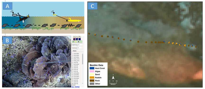
Figure 1: Georeferenced photoquadrat method principle. (A) Snorkeler, Diver or UW drone capture photoquadrats of the seabed. (B) Photoquadrats are analysed automatically in CoralNet for benthic composition, and (C) The analysed benthic composition for each photo is linked to its relevant GPS position and can be viewed as a pie graph overlayed on the satellite image.

Other methods for collecting new field data can include spot surveys (Roelfsema et al. 2006, Roelfsema et al. 2010), Remote Operated Vehicle (ROV) or Autonomous Underwater Vehicle (AUV) surveys (Roelfsema et al. 2015), and the utilisation of expert local knowledge (figure 2)

Figure 2: Variation of newly collected field data for the Allen Coral Atlas: (top left) Detailed surveys using our georeferenced benthic photoquadrat protocol: (top right) Basic surveys, characterising the benthos at one position: (lower left) Expert local knowledge: (lower right) remote surveys, where technology is deployed to gather autonomous information about the seafloor.

The georeferenced photoquadrat protocols are available online.  For a short overview of the photoquadrat method please see the protocol overview.  The full protocol, required software and assistance with training and site selection can also be provided if you are interested in collecting new data for the Atlas.   Since the start of the Atlas project various groups globally adapted the photo quadrat monitoring protocol and collected data in various countries: Fiji, Solomon’s, Philippines, Indonesian, Myanmar, French Polynesia, Palau, Red Sea, Kenya, Madagascar, Tanzania, Maldives, Bahamas, Belize, Porto Rico, Coral Sea, Jamaica, Cuba, Honduras.

Do you want to collect new data for the Atlas?

• Here is our global habitat mapping overview.   

2:  Existing benthic and geomorphic data and maps

Existing benthic and geomorphic data is also valuable to the verification process for both training and validation of the maps.  The habitat mapping team conducted extensive data searches for each of the mapping regions. Existing data is sourced utilising connections with local and international organisations and researchers active in each region, as well as internet searches for scientific and grey literature and available data and maps.  The benthic data collected are in various formats including existing maps, benthic transect data, and photoquadrats.  The collected data are cleaned, attributed to the required benthic classes, and summarised to the nearest geo-referenced point.  The data collection method and georeferencing accuracy is also recorded. 

Data requirements:

• Existing Field data.  Benthic data useful for the maps should be georeferenced, with a Latitude and Longitude provided for each sample point.  The data should describe benthic composition that could be collapsed to our general benthic categories (hard coral, soft coral, macroalgae, seagrass, sand, rubble, rock), with a documented survey method and date collected.
• Existing maps.  Existing maps should be georeferenced or able to be georeferenced and describe the geomorphic zonation and/or benthic composition.

All data contributed would not be published or used for any other purpose and will be acknowledged for the specific mapping region.

If you have benthic data for the coral reefs or seagrass habitats of your region, please consider contributing to the map training or validation process.  The more data we can gather for each region, the better the training and validation of those maps will be, resulting in more useful maps of the habitats in your region. 

Do you have existing data to contribute?

• Get in touch at submissions@allencoralatlas.org.
• For more information on mapping and monitoring through remote sensing from the University of Queensland, check out this Remote Sensing Toolkit

Reference

Roelfsema, C., M. Lyons, M. Dunbabin, E. M. Kovacs and S. Phinn (2015). "Integrating field survey data with satellite image data to improve shallow water seagrass maps: the role of AUV and snorkeller surveys?" Remote Sensing Letters 6(2): 135-144.

Roelfsema, C. and S. Phinn (2010). "Integrating field data with high spatial resolution multispectral satellite imagery for calibration and validation of coral reef benthic community maps." Journal of Applied Remote Sensing 4(1): 043527-043527-043528.

Roelfsema, C. M., M. Lyons, N. Murray, E. M. Kovacs, E. Kennedy, K. Markey, R. Borrego-Acevedo, A. Ordoñez Alvarez, C. Say, P. Tudman, M. Roe, J. Wolff, D. Traganos, G. P. Asner, B. Bambic, B. Free, H. E. Fox, Z. Lieb and S. R. Phinn (2021). "Workflow for the Generation of Expert-Derived Training and Validation Data: A View to Global Scale Habitat Mapping." Frontiers in Marine Science 8: 228.

 Roelfsema, C. M., S. R. Phinn and K. E. Joyce (2006). Evaluating benthic survey techniques for validating maps of coral reefs derived from remotely sensed images. Proc 10th Int Coral Reef Symp.

How can I learn more about the Atlas?

• Read our one-page overview: English - Spanish - French - Indonesia Bahasa
• Read our bleaching monitoring overview: English - Spanish
• Sign up for our newsletter
• Navigate to the Resources section of the website and explore our FAQ

How do I start using the Atlas in my coral reef work?

• Check out our demo video
• Take our online course, Remote Sensing and Mapping for Coral Reef Conservation
• Contact us at  support@allencoralatlas.org. We can offer guidance for integrating Atlas data into your work.

Do you have existing data to contribute?

• Get in touch at  submissions@allencoralatlas.org

Do you want to collect new data for the Atlas?

• Here is our global habitat mapping overview
• Here is our one-page summary of the data collection protocol

Keep scrolling down for more details!

On September 8, 2021 the Atlas completed the world's first global habitat maps, making the Atlas the first comprehensive mapping and monitoring system of coral reefs. These global habitat maps were updated with improved accuracy in late 2022.

Field Engagement team goals

The goal of the Allen Coral Atlas Field Engagement team, based at the National Geographic Society, is to help realize the vision of the late Dr. Ruth Gates of enhancing our collective ability to globally monitor, manage, and protect our unique and vibrant coral reef and coastal ecosystems.  We strive to get the Atlas into the hands of coral reef conservation practitioners, coastal communities, and coral reef scientists worldwide.

The Field Engagement Team’s purpose is threefold:

1. To raise awareness about the Atlas maps and products, and develop capacity within the conservation sector to utilize the tools and resources

2. To assess the uptake and impact of the Atlas as a tool to improve conservation efforts and inform management strategies and policies regarding coral reefs 

3. To facilitate the collection of new and existing data through an interconnected network of managers, researchers, and other organizations

Ultimately, the Atlas can help report on progress toward achieving international targets such as the Sustainable Development Goals and Convention on Biological Diversity Aichi targets. We are working with existing efforts (e.g., the International Coral Reef Initiative, the Global Coral Reef Monitoring Network, and the Reef Resilience Network) to facilitate planners, managers, and policymakers using the findings and data from the Allen Coral Atlas to achieve conservation impact.

How do I start using the Atlas in my coral reef work?

Whether you are a reef manager looking for habitat maps of your region to site areas for restoration, a researcher planning an expedition, a policy maker prioritizing coastal areas for protection, or you’re doing other work in need of spatial mapping of coral reefs, the Atlas can help. To get started, check our seminar with the South Pacific Regional Environment Programme, SPREP,  The Allen Coral Atlas: A new map for coral conservation (passcode: 5$CtuBX?) for an introduction to the Atlas and see how it is being used by NG Explorer, Patrick Small-horn West. You can also explore our Youtube channel. We created an online course on using the Atlas in collaboration with the Reef Resilience Network, read more and enroll here: https://reefresilience.org/remote-sensing-and-mapping/.

Photo by Michael Markovina 

Help us improve the Atlas

The Allen Coral Atlas is made possible by an enormous collaboration of organizations, agencies, and individuals. We rely on valuable input from scientists and managers to make the Atlas the best possible global tool.Unfortunately, errors are likely in a semi-automated machine learning process. That said, the mapping team will attempt to address reoccurring errors.

Photo by Team Lamu, CORDIO

Therefore, if you have identified a specific error on the Atlas, please write feedback@allencoralatlas.org and include:

• Reef name(s) or location either:
  • Copy URL of 'zoomed in' location
  • Coordinates and/or a georeferenced polygon (in KML, shapefile, or JSON format)
  • Screen shots from the Atlas of relevant area (annotated with details)
• Explanation of the error and your suggestion for correcting it/them
• Send us any relevant field data
• Contact details

Photo by Michael Markovina

Resources

Online Course - Reef Resilience Network

• Read more about remote sensing and mapping and the Allen Coral Atlas: https://reefresilience.org/remote-sensing-and-mapping/
• Enroll in the course:
  • English:  https://www.conservationtraining.org/course/view.php?id=950
  • Spanish:  https://www.conservationtraining.org/course/view.php?id=1105
  • French:  https://www.conservationtraining.org/course/view.php?id=1104
  • Bahasa Indonesia:  https://www.conservationtraining.org/course/view.php?id=1107

Habitat Mapping Protocol Information

• Dive and Snorkel Demo Video
• Short How-to Video

Check out Atlas GIS Tutorials

• Click on the Allen Coral Atlas Resources tab > Education > Technical Tutorials

Managed by UNEP-WCMC and IUCN, Protected Planet is the global authority on protected areas and other effective area-based conservation measures (OECMs). While their database spans the globe and includes marine and terrestrial datasets, the Atlas only displays marine protected areas relevant to the tropical coral reefs that we monitor. Thus, areas falling at least partially within 30 degrees North and 30 degrees South of the equator, and areas that are predominantly over saltwater are included for visualization on the Atlas. Protected areas for which the WDPA only has a point location have been approximated by drawing a circle around that point. All “statuses” delineated by the WDPA have been included. More detailed information on the WDPA’s categories can be found in the Protected Planet user manual. As per the terms and conditions of use of the database, protected area data is not downloadable from the Atlas but can be downloaded directly from Protected Planet’s website. Any errors in the data or questions should be directed to Protected Planet, as the data displayed on the Atlas website is sourced directly from Protected Planet.

UNEP-WCMC and IUCN 2023, Protected Planet: The World Database on Protected Areas (WDPA), updated monthly, Cambridge, UK: UNEP-WCMC and IUCN. Available at: www.protectedplanet.net.

National maritime boundaries are sourced from Marine Regions, a geospatial database managed by the Flanders Marine Institute, whose self-stated purpose is to “create a standard, relational list of geographic names, coupled with information and maps of the geographic location of these features”. While their database spans the globe, the Allen Coral Atlas only displays Marine Regions’ “Exclusive Economic Zone (EEZ)” dataset for areas that are indicated as “current”, and data points relevant to the tropical coral reefs that we monitor. Thus, areas falling at least partially within 30 degrees North and 30 degrees South of the equator are included for visualization on the Atlas*. Marine Regions’ EEZ dataset also includes UNCLOS-defined Territorial Seas, Internal Waters, and Archipelagic Waters designations, and water-emerging seamount areas may be excluded. The Allen Coral Atlas makes no determination on country sovereignty. Any errors in the data or questions should be directed to Marine Regions, as the data displayed on the Atlas website is sourced directly from Marine Regions.

More detailed information of the methods to designate boundaries can be found on Marine Regions’ methodology page and more information on maritime boundary designations can be found at the UN Convention on the Law of the Sea website.

*Please note that this means the statistics for an EEZ that partially crosses the 30 degree boundary may not fully represent the habitat there. For example, while we display the entire EEZ of Australia, we are only able to map tropical coral reefs up to 30 degrees latitude, and so any coral reefs (i.e. cold water corals) within that EEZ will not be captured.

Flanders Marine Institute (2022): MarineRegions.org. Available online at www.marineregions.org.